View and Work with 3D Point Clouds in QGIS

Introduction

In recent years, both government and private organizations have been putting point cloud data to use in many fields, including construction, disaster prevention, archiving, and infrastructure maintenance. Toward realizing digital twins built on point cloud data, several municipalities have also released prefecture-scale point cloud data as open data.

Analyzing this data in depth requires specialized software. QGIS, however, lets you view point cloud data and do simple processing on it with the same operations you use for ordinary layers.

This article uses point cloud data released as open data to explain how to display and process point clouds with standard QGIS features.

Point cloud data and QGIS

What is point cloud data?

Point cloud data is a collection of many points in three-dimensional space. Each point has coordinates that define its position with three values, (x, y, z). A point may also carry attribute information, such as color (R, G, B) and reflection intensity. Point cloud data is used in many settings, including terrain analysis, forest measurement, and modeling of buildings and objects.

Published point cloud data

Some municipalities publish point cloud data as open data. Portal sites for GIS data, such as the G-Spatial Information Center, offer point cloud data released as open data and also paid point cloud data.

• Tokyo Metropolitan Government Open Data Catalog Site
• VIRTUAL SHIZUOKA
• Open Nagasaki
• Wakayama Prefecture Geographic Information System
• G-Spatial Information Center

Note that this data is provided for a fee, but the Ministry of Land, Infrastructure, Transport and Tourism publishes 3D point cloud data for national highways under its direct control to make road management more efficient. At the time of the press release (August 2022), the data covered about 9,000 km, but as of October 2024, data for about 21,000 km is available.

The following site lets you browse the sections where the data is published. To use the data, download the application form (提供申込書), submit it, and complete the required procedures. (For details, see the website of the Japan Digital Road Map Association.)

Point cloud support in QGIS

QGIS supports point cloud data in the Entwine Point Tile (EPT) and LAS/LAZ formats. EPT is a format that splits point cloud data into hierarchical tiles so the data can be delivered and displayed efficiently. VIRTUAL SHIZUOKA and Open Nagasaki publish data in LAS format. QGIS always stores data as EPT, so the first time you load LAS/LAZ data, QGIS converts it to EPT. For processing, the QGIS 3.32 update added three lists to the Processing Toolbox, Point cloud data management, Point cloud extraction, and Point cloud conversion, which made basic processing possible.

Adding point cloud data to QGIS

Downloading point cloud data

First, download some point cloud data.

This article uses data published on Open Nagasaki, specifically the data around Oura Church (official name: Basilica of the Twenty-Six Holy Martyrs of Japan) in Nagasaki City, Nagasaki Prefecture.

On Open Nagasaki, the download page lets you download data by map sheet. Click the map sheet for the area you want to select it. The sheet number (here, “01KE9843”) and the size of the data to download then appear in the list of selected files (選択中のファイル一覧). On Open Nagasaki, the largest file in the currently published data is reportedly 685 MB. When you have selected all the map sheets you need, click Download (ダウンロード).

Adding point cloud data

Now add the downloaded point cloud data to QGIS.

The downloaded data is a ZIP file. On Windows, right-click the file and select Extract All. On a Mac, double-click the file to unzip it.

To add the data, drag and drop it from File Explorer, as you would vector and raster data. Or go to Data Source Manager → Point Cloud, browse to the location where the data is saved, and select the data you want to add.

The data you downloaded is now added. The point cloud data around Oura Church in Nagasaki City, Nagasaki Prefecture appears.

In 2D, the loaded point cloud data looks like a satellite image. But open a 3D map view with View → 3D Map Views → New 3D Map View and look at it in three dimensions, and it is clearly 3D point cloud data. Even trees and the cranes in the port area are captured in detail, not just buildings.

You can check the attribute information for the layer as a whole in Layer Properties → Information tab. Unlike a vector layer, you cannot open an attribute table to check information on individual points.

Setting the symbology

You can set the symbology of point cloud data in Layer Properties → Symbology tab. Choose from four renderers: Extent Only, which shows only the bounding box of the data; Attribute by Ramp, which draws points on a color ramp gradient defined by the maximum and minimum values of an attribute; RGB, which draws points with red, green, and blue color values; and Classification, which draws each class in a different color.

When data is added, QGIS selects the most suitable renderer by default based on the attributes the data has. This is a handy feature: data can be visualized just by adding it to QGIS, whatever its attributes.

• If the data contains red, green, and blue color information → RGB
• If the data contains a classification attribute → Classification
• Otherwise → rendering based on the Z attribute

Processing point clouds

QGIS provides three lists of processing tools for point clouds, Point cloud data management, Point cloud extraction, and Point cloud conversion, so you can do basic point cloud processing in QGIS.

Here is a quick look at what these tools offer. This article does not try each tool. On this site, the “QGIS X.XX New Features” articles in the blog introduce the features added with each version update. The articles tagged “#Point Cloud Data” show how point cloud features have expanded over time, and they are worth a look!

Point cloud data management

Vector data you usually work with is often measured in kilobytes or megabytes, but point cloud data often runs to gigabytes or terabytes. Adding such files to QGIS to display, process, and analyze them is not practical.

In that case, loading the data as a virtual point cloud (VPC) solves the file size problem. A virtual point cloud is split into tiles, and the part of the data needed for drawing is referenced from the actual files and displayed. This makes it easy to display and process large point cloud data.

Now try it. The data is part of the “LP Data Original Data” (LPデータ オリジナルデータ) from VIRTUAL SHIZUOKA Point Cloud Data for Central and Western Shizuoka Prefecture, published on the G-Spatial Information Center. Downloading it saves a ZIP file. As with the Open Nagasaki data, unzip it and you can confirm that LAS files were downloaded.

Once the ZIP file is unzipped, add the downloaded data to QGIS. Show the Processing Toolbox and select Point cloud data management → Build virtual point cloud (VPC) to open the window.

For the input data, click the ... button → Add File(s) and select the ~.copc.laz file generated in the directory that holds the point cloud data you added to QGIS. QGIS generates this file automatically when it loads point cloud data, to improve loading speed and processing efficiency. Select options as needed, specify the destination, and click Run.

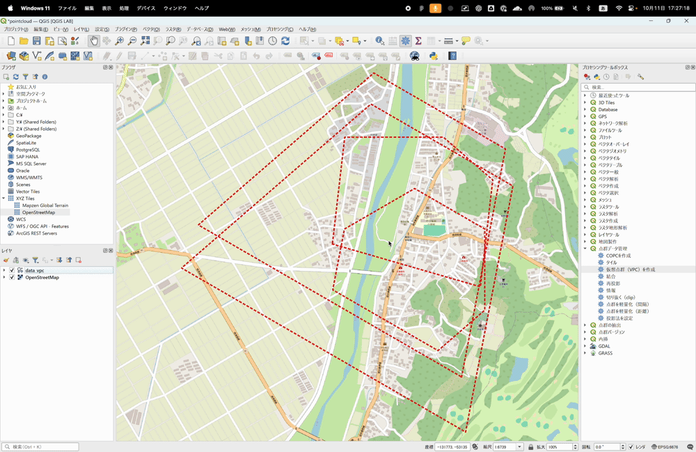
When processing finishes, the area that contains point cloud data is outlined with a red dotted line. Zoom in, and buildings, the ground, and other features are shown classified by color. Overlaid on OpenStreetMap, you can confirm that houses and other buildings are properly classified.

Select Layer Properties → Symbology → RGB, and the layer looks the same as when you added it to QGIS.

Other tools are available too. With Thin (by skipping points) or Thin (by sampling radius), you can thin out a point cloud at any interval or distance.

To combine multiple point cloud layers into one, use Merge. Note that the file size becomes larger.

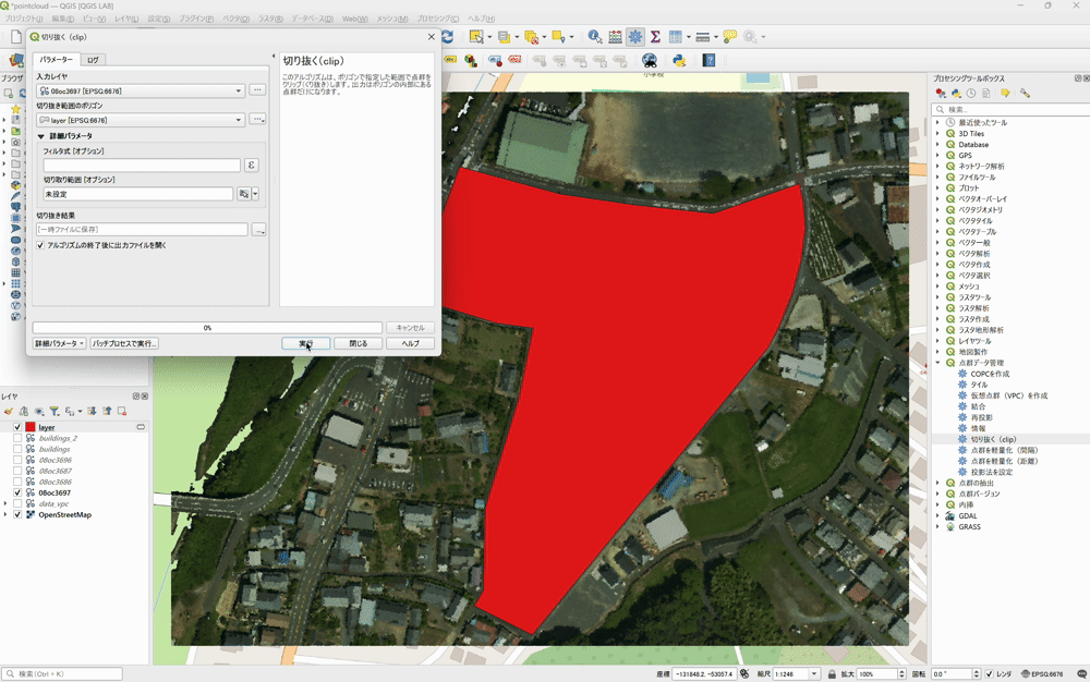
To clip a point cloud with any polygon, use Clip. It is convenient that you can clip with administrative area data or with a buffer around any point. As an example, a point cloud is clipped with a vector layer that traces the boundary of a residential area.

Point cloud extraction

The Boundary tool outputs a polygon that contains the topological boundary of a point cloud layer (topological here means spatial relationships such as contact, adjacency, and containment). In some cases, the output is a multipart polygon with holes.

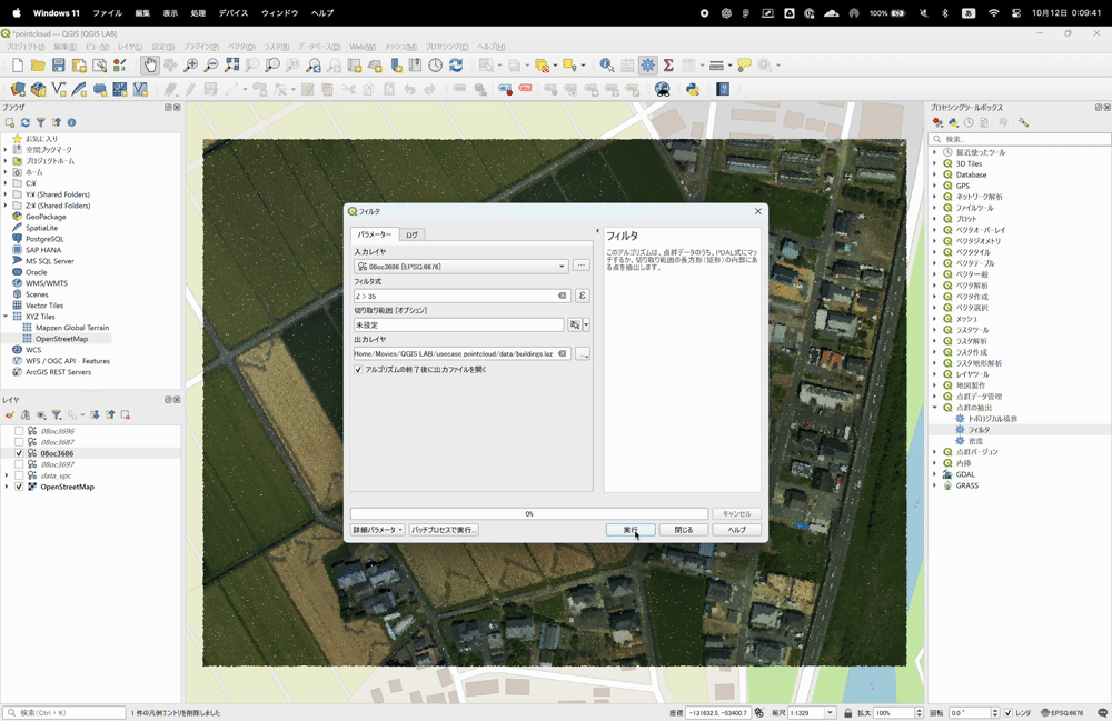
The Filter tool extracts the points that match a filter expression, or the points inside a specified cropping extent. As an example, filtering by the Z value (height information) in the attribute information extracted only the points that matched the condition (buildings). Compared with the original point cloud and OpenStreetMap, you can confirm that houses were extracted.

The Density tool outputs a raster layer that represents the density of a point cloud, using the specified point cloud layer as the area. It is a handy feature that lets you visualize the precision of the data easily and save it as an image.

The example uses the layer from which Filter extracted the buildings. Places with point cloud data (buildings) are colored lighter gray, and places without are colored black.

Point cloud conversion

The tools in the Point cloud conversion list change the format of point cloud data loaded into QGIS and output it.

With Convert format, you can output a point cloud layer in .LAS, .LAZ, .COPC.LAZ, or .VPC format.

With Export to vector, you can output point cloud data as a GeoPackage vector layer. You can optionally add attributes, and narrow the output by specifying an output extent or a filter expression.

Two tools export to a raster.

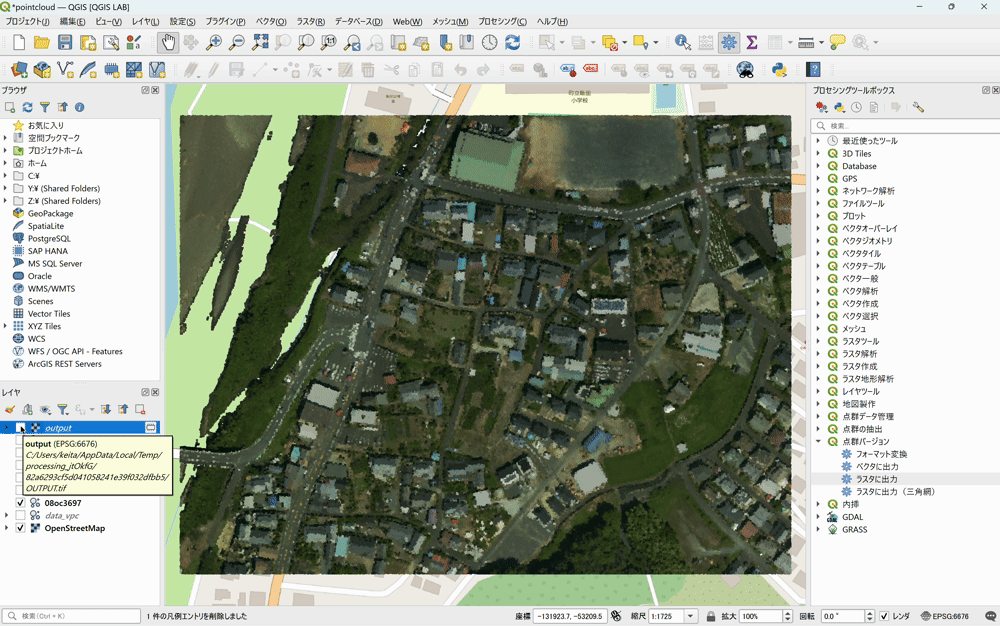
Export to raster exports a point cloud as a 2D raster grid whose cell size is the resolution you specify. Optionally, you can also assign the value of a specified attribute. Export to raster (using triangulation) connects the points with triangles to create a model of the ground shape or surface. Triangulation is an algorithm that generates a mesh made of triangles, and with this tool you can convert 3D information such as terrain into a 2D raster format.

As an example, the data was exported as a raster with Z (height) as the attribute and colored blue for lower values and red for higher values. The result visualizes the river as blue (low) and the trees as red (high).

Conclusion

Point cloud data tends to produce large files, but loading it as a virtual point cloud makes it easy to display in QGIS. You can also extract data by area or condition and export it in a different format.