
Noto Earthquake Laser Survey Data in QGIS
What you'll learn
- How to use airborne laser survey data related to the Noto Peninsula earthquake in QGIS
- How to add XYZ Tiles and vector tiles
- Steps to calculate DSM data from DEM and DCHM data
Recommended for
- Anyone who wants to analyze the latest aerial survey data in QGIS
- Anyone who wants to learn how to handle DEM and DSM data
- Anyone who wants to use GIS for disaster prevention and terrain analysis
Introduction

On March 19, 2025, the G-Spatial Information Center released various datasets based on airborne laser survey data collected jointly by the Forestry Agency and the Geospatial Information Authority of Japan (GSI). Besides helping with recovery and reconstruction from the earthquake, the data is expected to serve a wide range of fields, such as academic research for stronger local disaster prevention and new industries that use forest resources.
From the viewpoint of a user who works with the data, this article explains how to add the data to QGIS and how to calculate DSM data from DEM data and DCHM data.
Overview of the published data

Besides DEM data and DCHM data, the release includes topographic change data, collapse site interpretation results, and other datasets. All of them can be used in GIS.
| Data type | Overview | Data format |
|---|---|---|
| Forestry Agency: Digital Elevation Model DEM 0.5m (Noto Region 2024) | Data showing the elevation of the land | GeoTIFF, XYZ Tiles |
| Forestry Agency: Digital Canopy Height Model DCHM 0.5m (Noto Region 2024) | Data showing the height of each tree. It is the difference between the height of the surface, including trees and buildings, and the ground elevation at the tree locations | GeoTIFF, XYZ Tiles |
| Forestry Agency: Topographic Change Data (Noto Region 2024) | Data showing the difference in terrain before and after the earthquake | GeoTIFF, XYZ Tiles |
| Forestry Agency: Collapse Site Interpretation Results (Noto Region 2024) | Data showing the sites that collapsed in the earthquake | GeoPackage, vector tiles |
| Forestry Agency: CS Relief Map (Noto Region 2024) | A terrain map created by coloring elevation, slope, and curvature in separate color tones and overlaying them with transparency | XYZ Tiles |
| Forestry Agency: Forest Stand Type Map (Noto Region 2024) | An image showing the characteristics of tree species and crown shape, based on the canopy height, crown shape, and laser pulse reflection intensity acquired in the airborne laser survey | XYZ Tiles |
| Forestry Agency: Tree Species Polygons (Noto Region 2024) | Vector data that classifies the tree species, land cover, and so on that remote sensing technology can distinguish | XYZ Tiles, vector tiles |
| Forestry Agency: Simplified Orthophoto (Noto Region 2024) | A satellite image converted from a central projection by the lens to an orthographic projection viewed from directly above with no tilt | XYZ Tiles |
Adding vector tiles and raster tiles to QGIS
What is tile-format data?
Tile format means GIS data divided into small “tiles” of a fixed size and prepared in stages for each zoom level. It is less a new data format than a technique for delivering and displaying data efficiently.
GIS data comes mainly in two formats: raster data and vector data. Tile format splits each of them into tiles, and the results are commonly called “raster tiles” and “vector tiles.” Raster tiles suit basemaps and satellite imagery. Vector tiles are drawn on the client side (the user's device), so they allow more flexible operations, such as changing the style.

To learn more about GIS data formats, see the article below.
Connecting vector tiles
Next, connect vector tiles to QGIS.
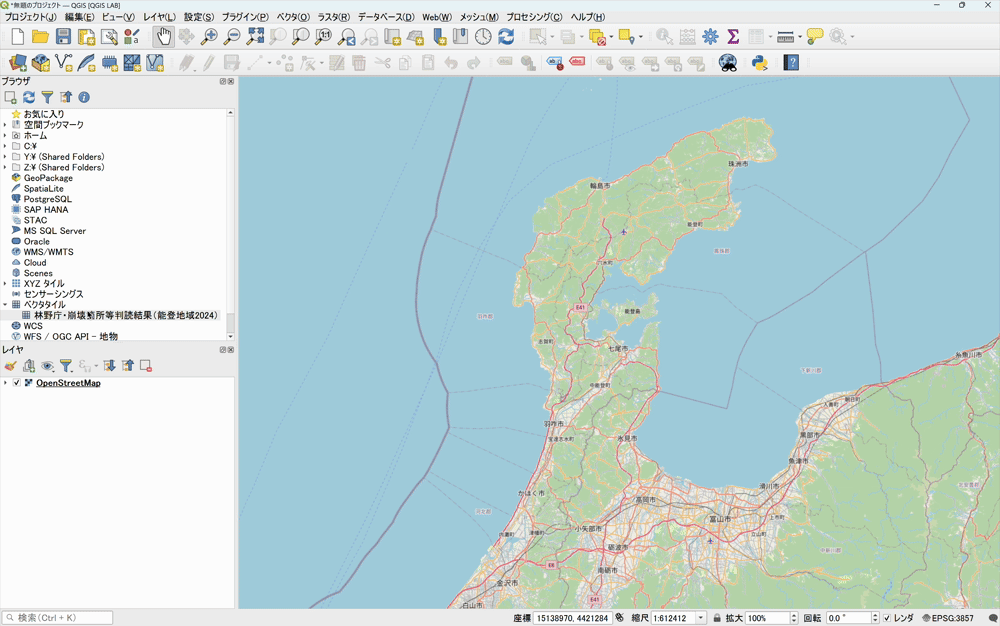
The data comes from “Forestry Agency: Collapse Site Interpretation Results (Noto Region 2024),” provided by the G-Spatial Information Center. Go to Details → More information to open the data details and find the URL for the connection. You also need the URL of style.json, so check that as well.

In QGIS, open the Browser panel and select Vector Tiles → New Generic Connection. The Vector Tiles Connection dialog opens.

Configure the settings as shown below to connect the vector tiles. Make sure no extra spaces come before or after the URLs.

- Name: enter any name
- Style URL: enter the URL of
style.json(the URL that ends with~style.json) - Source URL: enter the URL for Forestry Agency: Collapse Site Interpretation Results (Noto Region 2024) (the URL that ends with
~.pbf) - Set Min. Zoom Level and Max. Zoom Level (check the values with the data provider)
- Click the OK button
After you click OK, check that the vector tiles are registered in the Browser panel. Then double-click them or drag and drop them onto the map canvas to add them. Before adding them, it helps to display a basemap such as OpenStreetMap and zoom to the area you want in advance.
The vector tiles of the collapse site interpretation results now appear with their style applied.
Next, zoom in near the urban area of Wajima and view it in 3D with Qgis2threejs.
Landslides and cracks have occurred along the coastline and on mountain slopes. The main collapse areas stand out at mountaintops and on slopes, and deposition zones are spread across the gentler parts of the slopes.

For how to install and use Qgis2threejs, see the article below.
Connecting raster tiles
Next, add raster tiles to QGIS. The data comes from “Forestry Agency: Simplified Orthophoto (Noto Region 2024),” provided by the G-Spatial Information Center.
The connection works the same way as for XYZ Tiles, which are used for basemaps and similar layers. In the Browser panel, select XYZ Tiles → New Connection. The XYZ Connection dialog opens.
Configure the settings as shown below to connect the raster tiles. As with the vector tiles, make sure no extra spaces come before or after the URL.

You can add the raster tiles in the Browser panel to the map canvas by double-clicking them or dragging and dropping them. The published data is in WebP format, which has a higher compression ratio and a smaller file size than PNG, so maps load faster.

For details on adding XYZ Tiles raster tiles to QGIS, see the article below.
How to create DSM data
From here, the article explains how to calculate a digital surface model (DSM; “DSM data” below) from the GeoTIFF-format digital elevation model (DEM; “DEM data” below) and digital canopy height model (DCHM; “DCHM data” below), which are published alongside the tiles.
Raster tiles are easy to display, but because they are tiles, they are not suited to analysis. For analysis, use the GeoTIFF format.
Types of elevation data
First, a brief look at the types of elevation data. The published elevation data comes in two types: DEM data and DCHM data. These two datasets are used to calculate the DSM data.
The table below summarizes the differences between the elevation datasets.
| DEM data | DCHM data | DSM data | |
|---|---|---|---|
| Name | Digital elevation model | Digital canopy height model | Digital surface model |
| Height information | Elevation of the ground | Height of trees | Elevation including the height of buildings and trees |
| How it is derived | Ground elevation, obtained by removing the height of features from the surface height | Difference between the surface height and the elevation in forest areas | The surface height itself |
Import the DEM data and DCHM data into QGIS and add them together to create DSM data, an elevation model that includes the heights of buildings and trees. Unlike DEM data, the common type of elevation data, DSM data includes the heights of all structures on the ground, so it suits 3D analysis and similar work.

With this elevation data, you can carry out a variety of terrain analyses.
Downloading and adding the DEM and DCHM data
On the download page, the data is distributed under file names such as dem_07ED2.tif. A sheet index map is published to show which file covers which location, so check it.

This time, download the DEM data and DCHM data for 07ED3, which includes Wajima, and add them to QGIS by dragging and dropping.
Once added to QGIS, the data looks like this.

Calculating DSM data with the Raster Calculator
As noted above, DSM data comes from a simple calculation: DEM data plus DCHM data. To do the calculation, choose Raster → Raster Calculator from the menu bar.

When the Raster Calculator opens, select values from Raster Bands and Operators so that the Raster Calculator Expression box reads DEM + DCHM. If the expression is correct, Expression valid appears below it. After you enter the expression, click the ... button next to Output layer to set where to save the result. When all settings are done, click the OK button at the bottom.

A “Calculating raster expression...” dialog appears, and when processing finishes the DSM data is added to the map. At a wide scale, it looks fairly similar to the DEM data.

To check the result in detail, zoom in to an area with buildings and trees (near Wajima City Hall), style the DSM data with a gradient from red to blue according to elevation, and compare it with the simplified orthophoto.
The comparison shows that the data holds elevation values that include the heights of buildings and trees.

Switching the style to Hillshade also makes the three-dimensional look of buildings and trees clearer, which makes it easier to grasp surface conditions.

Viewing the DSM data in 3D
Finally, use the Qgis2threejs plugin to display the DSM data and the simplified orthophoto in 3D.
In the Layers panel, show only the simplified orthophoto and launch the plugin. Then, under Layers at the upper left of the window, check the “DSM data” layer. After a moment, an image like the one below appears, showing a 3D view that includes the heights of buildings and trees.

Overlaying the vector tile data from “Forestry Agency: Collapse Site Interpretation Results (Noto Region 2024)” mentioned earlier also lets you check the damage three-dimensionally.

Displaying DSM data in 3D like this represents the terrain more realistically.
Conclusion
This article used the airborne laser survey data released to examine the Noto Peninsula earthquake. It explained how to display the various tile datasets in QGIS, and how to create DSM data from DEM data and DCHM data and display it in 3D.
Combining DEM data and DCHM data makes it possible to grasp terrain in three dimensions, including the heights of trees and buildings. This kind of analysis can be used in many situations: creating three-dimensional terrain maps like the one in this article, analyzing three-dimensional changes in urban space, and terrain analysis such as measuring terrain displacement during a disaster.

QGIS LAB is a comprehensive information hub for QGIS, the open-source GIS software. Under the concept of “Geospatial for Greater Good,” we share the knowledge and skills to open up the world through location data.


